Comparing Propensity Modeling Techniques to Predict Customer Behavior

October 7, 2021Andrew Millett

A/B tests play a significant role in improving your digital experience. But A/B tests bring an inherent level of risk. There’s always a chance that the A/B test will have no significant results. In order to reduce the risk, propensity models can provide insights into which factors are worth investigating. While the models used in propensity modeling have been around for a long time, they recently have been picked up in the machine learning and e-commerce space.

Propensity Modeling Techniques Used for Decision Making

The term “propensity model” is a blanket term that covers multiple different statistical models that each are typically used to predict a binary outcome (something happens, or it doesn’t). For the purpose of guiding A/B tests, these propensity modeling techniques can also tell us which variables are indicative of users making a purchase. We can then devise an A/B test that modifies these variables for future customers. We will look at several different propensity modeling techniques, including logistic regression, random forest, and XGBoost, which is a variation on random forest.

For each model, we won’t dive deep into the math of it here but will give the pros and cons of each and provide links to resources as needed.

Logistic Regressions

The most “basic” of these propensity models, logistic regression, has been used in experimentation for a long time. While the application of the model and the interpretation of it is fairly straightforward, the math behind it can be somewhat complex. If you’re interested, visit this guide on interpretable machine learning.

Pros:

• Interpretable – Each feature gets a coefficient that can mathematically be tied to an effect. It also gives significance levels for each feature immediately, as well as positive or negative effects.
• Fast – The linear algebra used to calculate a logistic model is fairly simple.
• Accuracy – High accuracy on simple data.

Cons:

• Needs a simple, cleaned data set – Works best with linearly separable data (can draw a line between groups), and when there is no collinearity between features (two features are related).
• Mathematical explanation of the result can be difficult – Regular regression just has a numeric relation. Logistic does have to be transformed and is explained in “odds,” which isn’t always intuitive.

Random Forest

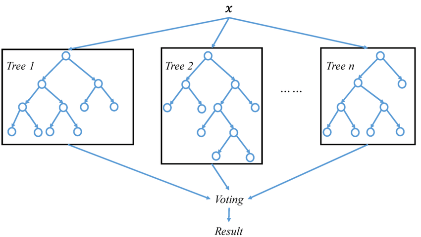
Another propensity modeling technique, called random forests, are computationally more complex than logistic regression, but the math is actually fairly straightforward. Random forests are “ensemble models,” which means it is made up of individual “learners” that then come together for a single decision. If you need more information on random forests and decision trees, you can review this beginner’s guide. Below is a visual representation of a simple random forest:

Random Forest Model (Source)

Pros:

• Adaptable – This model is known as a catch-all for basically any classification problem. Random forests will work fairly well regardless of data type, and this doesn’t require one-hot encoding and such.
• Robust – Handles outliers, includes a high number of features, and has non-linear relationships.
• Implicitly performs feature selection – Feature selection can be a time-intensive part of creating models, however, each decision tree is built with a random subset of features, and thus each trees performance is different.

Cons:

• Cost intensive – Can take a long time to run for large data sets.
• Black box – Very little control over what the model does beyond some hyperparameters (number of trees, max tree depth), and it’s very difficult to see why certain trees performed better/were given higher weights.

XGBoost

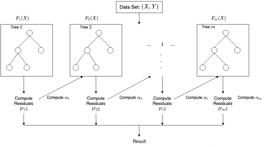
XGBoost is a propensity modeling technique that’s similar to a random forest in that it’s also an “ensemble learner” that uses decision trees. The difference is that random forests create hundreds of trees all at once and use all of them. Gradient boosting starts with one tree and adds a new learner in order to minimize the error. In essence, each new learner is supposed to fix the errors of its predecessors. For more information about XGBoost, visit the XGBoost Documentation. This process of adding a tree can be shown below. Note the difference between this and random forest. For XGBoost, each tree is computed only after the previous tree is done and the error is calculated so the new tree can address it:

Representation of XGBoost (Source)

Pros:

• Accuracy – Generally more accurate and less prone to overfitting (memorizing the training data, and thus performs badly when applied to new data).
• Speed – Runs faster than random forests.

Cons:

• Black box method – Difficult to interpret.
• Requires numeric variables – One-hot encoding is necessary.
• Harder to tune – There are more hyperparameters that can be changed for XGBoost.
• Have to define some loss function – Must define your error measurement, which adds to the complexity. Different loss functions may result in slightly different models when tuning hyperparameters.

Propensity Modeling Example Using Google Analytics Data Sample

Next, we’ll be looking at a sample data set that can be used with these different propensity modeling techniques. As many companies leverage Google Analytics (GA) to track data across their website, we’ll use a public data set in BigQuery. Specifically, the project “bigquery-public-data,” and the data set “google_analytics_sample.” This data is a brushed version of the Google Analytics data for the Google Merchandise Store. Not every field is available (lots are just filled with “not available in demo dataset”), but there’s enough to get user-level features and predict whether or not a user will make a purchase. This data set is available to anyone who has an account set up in BigQuery, so you can pull this exact data set and even add features if you want.

The features that we pulled are how many sessions, page views, and hits each user had, as well as the traffic mediums and device categories each user used. These categorical variables (medium and device) were one-hot encoded. This means that, instead of one column of data with multiple values (direct, organic, etc.), we make a column for each possible value. For example, there are four mediums in our data set: direct, organic, referral, and other. We’d then have four columns, and if the user had a direct traffic session, the “direct” column would have a 1, and the other columns have a 0. If a user had both referral and organic, then those columns would have a 1, while direct and others have a 0. See below for a simple example:

One-hot encoding (Source)

The SQL code we used to pull the data and perform the one-hot encoding is as follows:

There’ll be some slight modifications and data cleaning that’ll be done in R in order to help the propensity modeling techniques perform to the best of their abilities. This includes filtering missing data, undersampling, and reversing one-hot encoding for the tree-based propensity modeling. This sort of data wrangling should be expected for every machine learning process.

There are a couple of things that need to be done to the Google Analytics data that’ll help all models. The first thing that was done was removing the visitor IDs from the data set. This should be done for every data set used in machine learning. The “device_tablet” column could be inferred from the “device_mobile” and “device_desktop” columns, as there were only three device types for this data set. If there’s a 0 in mobile and desktop, there has to be a 1 in tablet. And if there’s a 1 in tablet, there has to be a 0 in mobile and desktop. This situation is called “linear dependence.” One of the requirements of logistic regression is that all the variables are independent, so we remove the “device_tablet” column as it’s redundant. This should also help clean up the data for random forests and XGBoost. We also encoded “transactions” to either be a 0 or 1, instead of allowing a user to have multiple purchases. We want to know “Do they make a purchase or not?,” not “How many purchases do they make?”

The final thing we did for universal cleaning is a process called “undersampling.” We’re looking at online transactions, which happen much less often than a user not making a purchase. In our case, purchases are made about 3% of the time. This means that even the simplest model that just assumes that no purchase is made is correct 97% of the time, which isn’t helpful. What undersampling does is randomly selects a subset of the more dominant result (no purchase) so that there’s an even split of purchase and non-purchase users. This allows models to have a better chance to learn the features that actually matter in determining the likelihood of a purchase. This also reduces the size of the data set, so the models run faster. Of the 186,000 observations from 2017, we end up with 11,000 observations to use for our propensity modeling with an even split of purchasers and non-purchasers.

Propensity Modeling Performance

With the majority of the data cleaning finished, we can move on to training our models and evaluating how they compare to each other.

Logistic Regression

With the data cleaning done, we first look at the logistic regression model. The Google Analytics data at this point is clean enough to be put into a model, so we split our data into training and validation sets. We do this to ensure the model still performs well when it’s introduced to new data. The “standard” amount is to train on 70% of the data and validate with the remaining 30%. We then train the model on the training data set so it can learn which features are indicative of making a purchase.

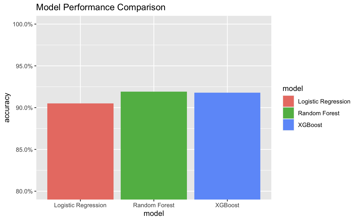
We found that the more pageviews (using a desktop) and actually fewer sessions indicated a user would make a purchase. We then have the model predict whether the remaining 30% made a purchase. We were able to achieve a 90.5% accuracy for our model. This means, of the 3340 new users, it misclassified 317 of them.

Random Forest

Next is the random forest model. We mentioned earlier that we did some one-hot encoding for the categorical variables so the logistic regression model would perform better. However, it has been found that random forests perform worse with one-hot encoding. As such, we’ll want to revert the one-hot encoding. This means putting the broken-out medium columns into one categorical variable, as well as the devices. The rest of the data stays the same, which means we can again create our 70%-30% training and validation split.

While we can’t see which variables had a statistically significant impact on estimating purchase like we can with the logistic model, we still can see the “importance” rank of each variable. In this case, the number of sessions, page views, and hits (pageviews and events) were the most indicative of making a purchase. Unlike the logistic regression, we don’t know if these have a positive or negative relationship, just that they were important to making the prediction. When we validated the model, our random forest had an accuracy of 91.9%, misclassifying only 270. This could likely be refined further by changing some of the hyperparameters, but we went with the default settings in R for this case.

XGBoost

Finally, we can evaluate the XGBoost model. Even though the structure of XGBoost is similar to that of the random forest, the data structure required is closer to that of the logistic regression model, so we’ll use the data set that has one-hot encoding. There are also many hyperparameters we could tweak for XGBoost, as well as choosing one of several “loss functions,” but we’ll keep the default settings and loss function (in this case, the log-loss).

With as simple a model as we can get, we achieved an accuracy of 91.8% when predicting the outcome for the validation set. This means 274 were misclassified, just a few more than the random forest. Again, we could change our hyperparameters and likely improve this performance, but that won’t be covered in this article. Similar to random forests, we can get the ranked importance of the features used. For our model, number of page views, time on site, and a desktop device were the highest indicators of making a purchase. Below, you can see the performance of all three models side by side.

Figure 1: Model Accuracy

Analyzing the Results of the Propensity Modeling Techniques

For the data set, we had using public Google Analytics data from BigQuery, the random forest model performed the best (though by a small margin). But here’s an important note: random forests will not be the best models in all situations. There’ll never be a machine learning model that is the golden snitch, that will ensure perfect results every time or perfectly describe customer behavior. To quote statistician George E. P. Box, “All models are wrong, but some are useful.” In other words, every model has its limitations, and you often need to try several different models and compare their performance to find the best model for that specific situation.

There’ll never be a machine learning model that is the golden snitch, that will ensure perfect results every time or perfectly describe customer behavior Click & Tweet!

It’s also wise to keep in mind the end goal of using any of these predictive model techniques. While it’s valuable to try to predict whether a customer will convert, these models won’t predict the outcome of actions taken after the prediction is made, such as a follow-up email. Always check the model to see which features were influential in the model and use that to guide your next actions and A/B tests. As we were looking to see what factors had an impact on a user’s likelihood to convert and not the likelihood prediction itself, we may be more likely to use the logistic regression propensity modeling technique despite its lower accuracy. Each case will be different.

Do you have an upcoming A/B test that you’d like to prepare for? Blast specializes in helping brands improve their digital experience backed with statistical rigor to ensure the best results.

About the Author

Andrew Millett

Andrew Millett is a Data Analyst at Blast Analytics. He has worked with clients such as Kontoor, Fracture, and Keurig, where his experience with R and statistical methods helps find answers to key business questions. He's constantly striving to learn and use new statistical methods to provide insights that improve the digital customer experience.

Connect with Andrew on LinkedIn. Andrew Millett has written 2 posts on the Blast Digital Customer Experience and Analytics Blog.